Today I saw a hourly weather radar forecast, showing a storm front passing through. But there was an interesting artefact you’ve probably seen before and not paid much attention to. The rain bands teleport across the map, fade out, and teleport again. Looking at the results, it’s pretty obvious how this works. Every point on the map had its values interpolated between discrete forecast steps independently of all the others.
How can we get an interpolation that looks like smooth continuous motion of a single object rather than fading between three photos of separate objects? I’m not sure exactly, but it sounds like great fun to try.
What others are doing
Video Compression
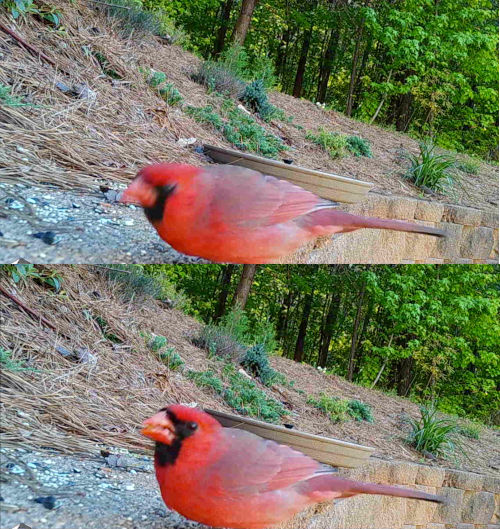
The most direct example I can think of where this is already done is in video compression. To keep the video crisp, the shutter needs to be open as small a fraction of the time as possible, to freeze action on each frame. While the angular resolution is awesome in these situations, the time resolution is generally the same ~24-30hz, with some exceptions. This means there can be fairly large changes between consecutive frames, such as this cardinal from my backyard. It pretty clearly show that a linear mix is going to look very strange.

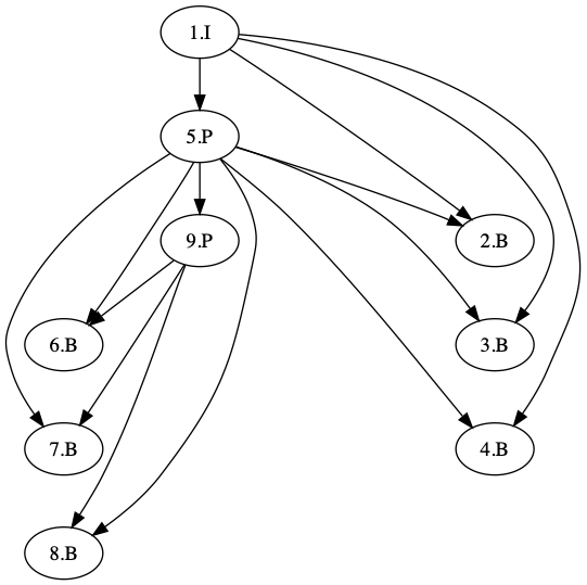
If someone did bother to interpolate between frames, you wouldn’t notice anyway because of flicker fusion. But actual video compression uses interpolation on a much larger scale. The default settings for x264 in VLC show that frames are encoded in groups of between 25 and 250, meaning at least around a second of images will be predicted from each other, and probably more like five seconds. It’s harder to say where the interpolations end though, because it does stretch intuitions about what interpolation means. A typical, but short GOP, might look like the following, where I frames are independent images (also called keyframes), P frames are “predicted” from their previous frame’s reconstruction, and B frames are predicted from their nearest I and P neighbors on both sides. B frames are not predicted from other B frames, so that way it’s safe for B frames to be lost. Since most frames are B frames, this improves fault tolerance quite a bit.
This doesn’t really answer the question, so far. The predict in an interesting network but how do they perform that prediction? Video compression is complex, but there are at least three different forms of compression going on under the hood that make this work.
- Spatially informed, temporally invariant lossy compression based on a frequency space transform (DCT), and truncation via quantizers (both in JPG)
- Several lossless statistical compressors like Arithmetic coding (as in GIF), Huffman trees (in PNG), and now CABAC (in several MPEG variants)
- Motion compensation, where the next image is constructed by moving regions (usually power-of-two squares) of the previous image spatially to minimize prediction error
Statistical compressors are quite interesting, but the two pieces we are after are the selective frequency filtering, and motion compensation. But I’m out of time for today so we’ll start looking over those tomorrow.